Robert Beard
Cracking Cracking the Coding Interview
Gayle Laakman McDowell’s wonderful Cracking the Coding Interview includes the following practice problem:
17.23 Max Black Square: Imagine you have a square matrix, where each cell (pixel) is either black or white. Design an algorithm to find the maximum subsquare such that all four borders are filled with black pixels.
The answer section provides two solutions:
- A simple brute-force solution where you check each pixel for possible squares in descending order of size. This solution is O(n4). There are n2 pixels that could be the top-left corner of a square, O(n) sizes of square to consider, and O(n) pixels on the border of such a square to check.
- An optimized algorithm that precomputes for each pixel the number of consecutive pixels to the right and down from each pixel in the grid. With these statistics in hand, it becomes possible to check for the existence of a square of size
sat a given point in O(1) time by looking at the top-left, bottom-left and top-right pixels and confirming that there are at leastsconsecutive pixels heading in the correct direction. This optimization improves the overall runtime to O(n^3): O(n2) top-left pixels to check, O(n) sizes of square at each pixel, and constant time to check each candidate.
Is the second solution the optimal one? Or as Tim Roughgarden often asks, “Can we do better?” As it turns out, no it’s not, and yes we can do better, by building on the precomputation approach of the second solution.1
The inefficiency in the second solution is that it checks for all possible squares of all possible sizes in brute-force manner. The method of checking whether a square exists is clever, but all possible squares are checked. This approach fails to make use of the full structure of the problem. To get some clues about how to improve it, let’s look more closely at how the algorithm proceeds.
The bones of the algorithm look like this. There’s a full working implementation of this algorithm (and the rest of the code discussed here) on Github, but the key ideas are below:
def find_largest_square(grid):
    pixel_runs = precompute_pixel_runs(grid)
    for size in range(grid.side_length, 0, -1):
        for pt in grid:
            if is_valid_square(pt, size, pixel_runs):
                return size
    return 0

def is_valid_square(top_left, size, pixel_runs):
    top_left_entry = pixel_runs[top_left]
    top_right_entry = pixel_runs[Point(x=top_left.x + size, y=top_left.y)]
    bottom_left_entry = pixel_runs[Point(x=top_left.x, y=top_left.y - size)]
    return (top_left_entry.right >= size and top_left_entry.down >= size and
            bottom_left_entry.right >= size and top_right_entry.down >= size)
Refactoring the precomputations
The first step in improving the algorithm is to rationalize the way we access the table of precomputed values. As it stands, we have to query three cells to determine whether a square is valid. At the top-left, we check both the down and right values against size. Then we check two of the other corners, but we only look at one of the two data values there. More specifically, we’re checking whether there’s a consecutive run of pixels from the checked point to the fourth corner of the potential square. Why not just store both pieces of information in the fourth corner and find it there? In other words, our new and improved precomputation table will include the length of the consecutive pixel runs going in each of the four directions from each pixel. With our new table, we can rewrite our square-existence test:
def is_valid_square(top_left, size, pixel_runs):
    top_left_entry = pixel_runs[top_left]
    bottom_right_entry = pixel_runs[Point(x=top_left.x + size, y=top_left.y - size)]
    return (top_left_entry.right >= size and top_left_entry.down >= size and
            bottom_right_entry.left >= size and bottom_right_entry.up >= size)
Also note that it’s superfluous to track right/down and left/up separately. We always look to see whether both of them are larger than the candidate size–why not just save the smaller of the two? Now our test function looks like this:
def is_valid_square(top_left, size, pixel_runs):
    top_left_entry = pixel_runs[top_left]
    bottom_right_entry = pixel_runs[Point(x=top_left.x + size, y=top_left.y - size)]
    return top_left_entry.right_down >= size and bottom_right_entry.left_up >= size
Thinking diagonally
What have we accomplished? So far, nothing. This is still an O(n3) algorithm. We just reshuffled the precomputed data to make it easier to think about. For further inspiration, let’s reorganize our core loop a little:
def yield_squares(grid):
    ...
    for pt in grid:
        for size in range(grid.side_length, 0, -1):
            if is_valid_square(pt, size, pixel_runs):
                yield size  # We'll need to collect these and find the max
All we’ve done is swap the outer two loops. This is less efficient on average, because we can’t return early as soon as we find a square, but it doesn’t affect the worst-case runtime, and it’s just a thought experiment. Now, let’s look at the table entries consulted in the first two iterations of the outer loop.
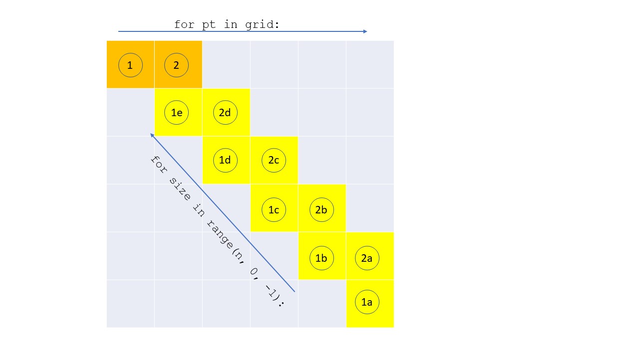
For the first point considered (orange, labeled with a 1), the table entry corresponding to the point being studied is consulted for each possible square. Then in each iteration of the inner loop, the yellow entries labelled 1a, 1b, etc., are consulted in order. On the next pass of the outer loop, the orange entry labelled 2 is consulted, and the corresponding yellow entries are looked at in a similar order. Now let’s skip ahead to the iteration #7 of the outer loop.
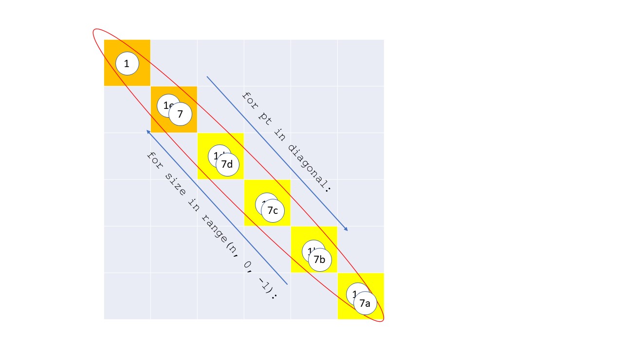
This picture highlights an important element of the problem’s structure. For any square whose top-left or bottom-right corner lies on a particular diagonal, all the information we need to know is embedded in that diagonal of our table. This makes sense if we think about our modified precomputation table. One of the numbers in each cell of the table stores the length of the shorter consecutive run of pixels going in the down or right directions, and the other stores the same figure for up and left. Geometrically, this number is the leg length of an L-shape with equal legs whose vertex is situated on that point of the grid and opening down/right or up/left, as the case may be. If we imagine two such shapes positioned on a diagonal, the significance becomes clear. If you move two L-shapes towards each other, they form a square the moment the legs on the shorter L-shape touch the legs of the larger one, which occurs when they are separated by an x- or y-distance equal to the leg length.
We can use these ideas to reshuffle our algorithm once again:
    for diagonal in grid:
        for p in diagonal:
            leg_length = pixel_runs[p].down_right
            for size in range(leg_length, 0, -1):
                q = Point(x=p.x + size, y=p.y - size)
                if pixel_runs[q].up_left >= size:  # key statement
                    yield size  # We'll need to collect these and find the max
Eliminating impossible squares
We still haven’t accomplished anything though–this algorithm is stubbornly cubic. We haven’t extracted enough structure from the problem. We’re still basically testing all P/Q pairs on a given diagonal. We save a little time by skipping Q candidates that are outside the arms of P’s L, but that doesn’t affect the asymptotic running time. We also need to prune based on the size of the up/left L at Q. To see how, let’s look at a particular point Q on the diagonal and see how the result of the inner if statement in the loop evolves as the outer loop looks at different candidates for P.
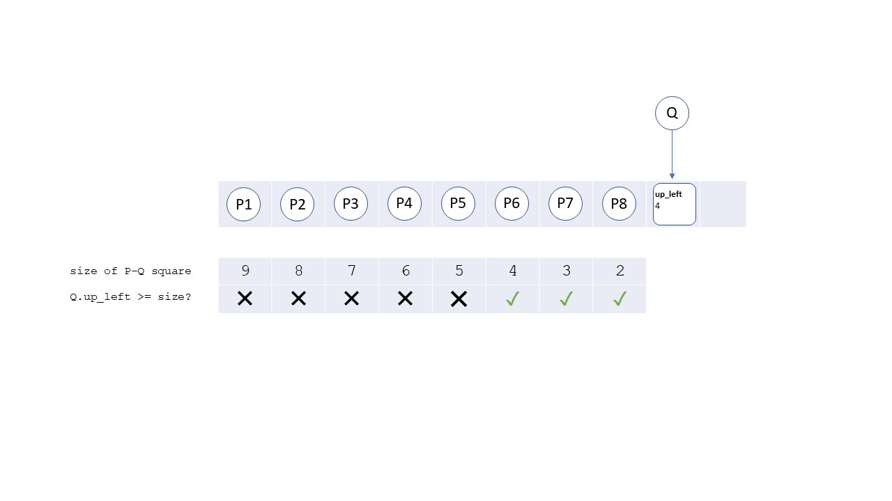
Well, that’s interesting! For a given point Q that gets tested against a bunch of Ps in sequence, the results follow a very predictable pattern. For Ps before a critical point, Q never makes a square because the up-left L isn’t long enough. After that critical point, Q makes a square with any P whose down-right L reaches Q. (Geometrically, the critical point is the top-left corner of the square made by filling in the L at Q.) So, why are we testing Q before that critical point? Instead of testing every candidate Q, we need to limit our search to only those Qs that reach P.
How do we do that? As with everything in this algorithm, the answer is preprocessing. For our first step, we are going to find the critical points for each Q in the diagonal. Then as we traverse candidates for P, we will build up a list of the Qs whose critical points are behind us.
    for diagonal in grid:
        critical_points = defaultdict(list)
        for q in diagonal:
            leg_length = pixel_runs[q].up_left
            critical_points[Point(x=q.x - leg_length, y=q.y + leg_length)].append(q)
        q_candidates = []
        for p in diagonal:
            q_candidates += critical_points[p]
            leg_length = pixel_runs[p]
            for q in q_candidates:
                if  0 < q.x - p.x <= leg_length:  # key statement
                    yield q.x - p.x
Are we there yet? Sadly, no. This is still O(n2) for each diagonal and O(n3) for the full problem. The reason is that scanning through our list of Q candidates is taking too long. That list can be O(n) long, so we can’t afford to do a full scan n times per diagonal. We need to be faster. To achieve this, we can rely on the fact that we don’t need to check every Q in the list. We just need to find the most distant Q that’s reachable from P. In other words, we want the reachable Q with the highest x-coordinate (or y-coordinate if you prefer). Since we start out with our list of points sorted by x-coordinate, binary search seems like a natural solution to this problem, and it’s fast. All we need to do is keep q_candidates sorted as we traverse the diagonal, then at each step we can do our lookups in log n time and get ourselves to a runtime of O(n log n) for each diagonal and O(n2 log n) for the full problem!
def yield_squares(grid, pixel_runs):
    for diagonal in grid:
        critical_points = defaultdict(list)
        for q in diagonal:
            leg_length = pixel_runs[q].up_left
            critical_points[Point(x=q.x - leg_length, y=q.y + leg_length)].append(q)
        q_candidates = []
        for p in diagonal:
            q_candidates = merge_sorted_lists(q_candidates, critical_points[p])
            farthest_reachable_x = p.x + pixel_runs[p].down_right
            best_q = find_max_lte(q_candidates, farthest_reachable_x)
            if best_q is not None:
                yield best_q.x - p.x

def find_max_lte(l, boundary):
    if not l or l[0].x > boundary:
        return None
    if len(l) == 1:
        return l[0]
    midpoint = math.floor(len(l) / 2)
    target_sublist = l[:midpoint] if l[midpoint].x > boundary else l[midpoint:]
    return find_max_lte(target_sublist, boundary)
This all looks very clever, but it still doesn’t work! We achieved our goal of finding the best square for each P in the diagonal in log n time, but we introduced a new problem. Now we’re doing too much work to maintain our sorted list of candidates. Merging lists is an O(n) operation, and we could have to do it as many as n times. No good.
Data structures to the rescue
We need a better data structure than the humble sorted array. More precisely, we need a data structure that still allows us to find an element (or its predecessor, if the element does not exist) in O(log n) time, while also allowing O(log n) insertions. A binary search tree (BST) fits the bill. Note, however, BST operations technically run in time proportional to the height of the tree. With efficient packing, the height of the tree can be kept to O(log n), but it requires some additional bells and whistles to handle pathological cases. See wikipedia for an explanation and a formidable list of jargon-y names for solutions. We could simply use an existing implementation of one of these solutions, or code one for ourselves, but I prefer a third option. For this problem, we don’t really need the full power of a self-balancing BST. Moreover, we have an important advantage, which is that we know the shape of the full BST after all the points on the diagonal are added. This bit of foreknowledge should allow us to skip all the finicky tree adjustments that are required for ongoing balancing and just start out with an optimally structured tree.
Here’s the idea. Rather than starting with an empty tree consisting of just a root node, we’ll use the sorted list of points on the diagonal to build a template for our data structure (which I’m going to call a skeleton tree–it may have a real name that I don’t know about). Then, as we encounter reachable Qs in our traversal of the diagonal, we’ll insert them into the tree in their appointed position. The trickiest part is ensuring that we support a quick search for a value’s predecessor. As a negative example, imagine we constructed a standard BST from our sorted list of points, then added a field inserted to each node in the tree (this field would be false for every node at the outset, because the tree is empty). When we encounter a new Q, we would just set inserted to true for the node that stores Q. This would allow quick insertions and lookups (just do a normal traversal to the place we expect to find the value and either set or read inserted, respectively). However, we could no longer easily find the predecessor of a value. In a standard BST, the process for this operation depends on being able to tell quickly whether the left and right subtrees of particular nodes are no longer empty. This is easy to do when an empty subtree is represented by the null value. With our skeleton tree, though, the left and right subtrees are never null, so we would need to traverse an entire subtree and see that it has no inserted values to conclude that it is empty.
Instead, we’ll make two modifications:
- We’ll store all values at the leaves. This is a little inefficient, but at least half of the nodes of a balanced binary tree are leaves, so it can’t be that bad.
- Now that we don’t need the internal nodes for values, we will use them to store two things: (a) the roadmap for filling in and querying the tree, in the form of the largest value that “belongs” to the left subtree, and (b) a flag that tracks whether the subtree rooted at that internal node is empty.
More specifically, when we initialize the skeleton tree, we’ll give each internal node with a field left_cap, which represents the largest value assigned to the left subtree and is equal to the median of the values stored in the subtree.2 We’ll also add a field is_empty which will be initialized to True. When we want to insert an element, we’ll traverse the tree, comparing the value to left_cap at each step. If the value is less than or equal to left_cap, we’ll proceed to the left child, otherwise we’ll proceed to the right. When we reach the bottom of the tree, we insert our value as the left or right leaf from the last node. During our traversal, we’ll also set is_empty to false for each node that we visit, since that node will now be the parent of at least one value.
To do a lookup, we follow the same process, except we can conclude that the value is not in the tree if we ever hit a node where is_empty is True. To find a value’s predecessor, we go to first empty node on the path to where that element should be. If that empty node is the right child of its parent, then the predecessor is the largest element in the left child of the parent. If the empty node is the left child, then we go up the tree until we find an ancestor node that is a right child and that has a nonempty left sibling, then we return the largest element in its left sibling.
Code for the skeleton tree is also on GitHub. Here’s the final algorithm in all its glory:
def find_largest_square_v2(grid):
    return max(yield_squares(grid))


def yield_squares(grid):
    ells = compute_ells(grid)
    for diagonal in grid.diagonals():
        diagonal = list(diagonal)

        critical_points = defaultdict(list)
        for q in diagonal:
            if leg_length := ells[q].up_left:
                critical_points[Point(x=q.x - leg_length + 1, y=q.y + leg_length - 1)].append(q)

        q_candidates = SkeletonTree.from_sorted_list(diagonal)
        for p in diagonal:
            for q in critical_points[p]:
                q_candidates.insert(q)
            farthest_reachable_x = Point(x=p.x + ells[p].down_right - 1, y=p.y - ells[p].down_right + 1)
            if (best_q := q_candidates.find_value_or_predecessor(farthest_reachable_x)) is not None:
                yield best_q.x - p.x + 1
The final runtime of our algorithm is O(n2 log n). Computing the size of the L-shapes is O(n2), which is done once for the whole algorithm. The meat of the algorithm runs once for each diagonal, of which there are O(n). In each loop, we compute the critical points (O(n) work), initialize the skeleton tree (O(n)). For each of the O(n) points on the diagonal, we do a lookup (O(log n)) and yield a single point (O(1)). The lookups end up being the bulk of the work, as we have O(n2) of them, and we take O(log n) time for each, which gives us our overall runtime. Note also that we don’t find all the squares in the grid. We don’t have time, because there could be as many as O(n3) squares.3 Instead, we’re just returning the largest square for each top-left in the grid.
Results
The Github repo includes some tests to build confidence that this algorithm actually works, as well as some very informal benchmarks against the algorithm from CtCI. The results bear out our expectations. For very small instances (n=10), the simpler algorithm is faster. In particular, on instances where most of the pixels are filled, the simple algorithm has a relative advantage, because it is more likely to find a big square and terminate early. Our algorithm has a more consistent running time, since it looks at every square no matter what. For somewhat larger instances (n=100), our algorithm has a speed advantage of between 2x (for a 95% filled grid) and 6x (for a 10% filled grid). For larger instances (n=800), the difference between an O(n) factor and an O(log n) factor becomes clear, and our algorithm is 50x faster for the sparsest instance and 25x faster for the 95% filled one. Note that the benefit of early stopping gets smaller and smaller as the problem size increases. The odds of making a filled square of size N from 4N - 1 random pixels arranged in the right way drops off exponentially as N increases (it’s just pfilled4N - 1) while the number of such arrangements only increases quadratically as the grid grows. This means that the largest square you can find in a 95%-filled 800x800 grid is not much larger than the one you can find in a 400x400 grid.
Final thoughts
I hope this was a fun exercise in optimizing an algorithm and stretching for optimal performance. (I have no proof that this runtime is optimal, but it feels like it should be.) Needless to say, I would not encourage you to try to design something like this in a technical interview–stick with McDowell’s proposed solution for that one.
-
While I don’t know for sure, I suspect that McDowell was aware of this solution, or at least that the optimal solution is not presented in CtCI. In describing the solutions to these problems, she assiduously avoids describing the fastest solution offered by the book as “optimal” or “optimized,” which she typically does when it’s true. I would speculate that the algorithm presented here was omitted because it’s way too elaborate for a solution to a whiteboard problem. ↩
-
Incidentally,
left_capturns out to be a hard field to give a good name to.midpointorsplit_pointare clear, but they don’t help you remember which side the midpoint value is stored on. A reader might expect a field calledleft_maxorlargest_left_valueto store the maximum value currently in the left subtree.largest_value_to_store_on_leftis clear and correct, but a bit too long for my tastes, at least in this situation.left_capis a bit meh, but I don’t think it does any active harm. ↩ -
This fact also misleadingly suggests that an O(n3) algorithm is the best you can do. The way out of that bind in this case is that we only need the largest square at each point to answer the problem presented. Once we know the size of the largest square, we don’t care if there are any smaller ones. ↩